결정트리
- Decision Tree는 데이터를 여러 규칙(if-then) 으로 분할해 나가면서 예측
- 데이터에서 가장 정보 이득(Information Gain) 또는 지니 지수(Gini Index), 카이제곱 통계량을 감소시키도록 분할
- 회귀일 경우 분산 감소(Variance Reduction)가 큰 변수를 선택 / F 통계량이 작아지도록 분할
- 정답에 가장 빨리 도달하도록 질문하는 방법을 학습
- 계단 모양의 결정 경계를 만들기 때문에 데이터의 방향에 민감 → PCA 변환 적용
- 상관성이 높은 다른 불필요한 변수가 있어도 크게 영향을 받지 않음.
- 수치형 / 범주형 모두 가능
ㄴ F통계량, 분산의 감소량 / 카이제곱 통계량, 지니지수, 엔트로피 지수
- 이상치에 민감하지 않음.
- 계산 복잡도 : 탐색 - O(log2m), 훈련 - O(n*m*log2m) / m = 훈련 데이터 수, n = 특성 개수
장점
해석 용이성
- 사람이 이해하기 쉬운 if-then 규칙으로 설명 가능 → "왜 이 결과가 나왔는지" 설명 가능(Explainable AI).
비선형 관계 처리
- 변수 간 선형 관계를 가정하지 않음.
전처리 간단
- 스케일링(Standardization, Normalization) 불필요
- 결측치 처리에도 비교적 유연.
범주형/연속형 변수 모두 처리 가능
- 혼합된 데이터도 자연스럽게 처리.
빠른 예측 속도
- 한 번 학습되면 예측 단계는 규칙 탐색이라 빠름.
단점
과적합(Overfitting)
- 트리를 깊게 만들수록 학습 데이터에 지나치게 맞추어 일반화 성능이 떨어짐.
작은 변화에 민감
- 데이터에 조금의 변화가 있어도 트리 구조가 크게 달라질 수 있음 (불안정성, 큰 분산).
- 분류 경계선 부근의 자료에 대해 오차가 증가
편향된 분할 가능성
- 클래스 불균형 데이터에서는 분할 기준이 한쪽으로 치우칠 수 있음.
복잡한 관계 표현 한계
- 단일 트리로는 복잡한 패턴 학습이 어려움 → 그래서 앙상블(랜덤 포레스트, XGBoost) 기법이 많이 사용됨.
- 설명변수 간의 중요도를 판단하기 어려움
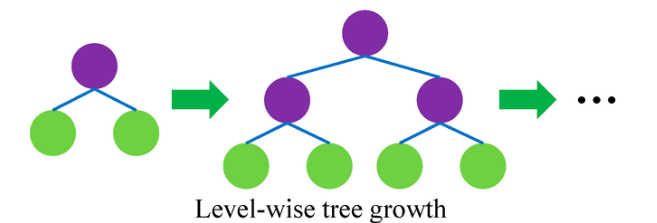
결정트리 성장 방식 비교
레벨 기준 성장 (Level-wise / Breadth-first)
- 트리의 깊이를 일정하게 맞추면서 같은 레벨의 노드를 동시에 분할
- ex. 모든 노드를 깊이 1까지, 그다음 깊이 2까지 … 확장
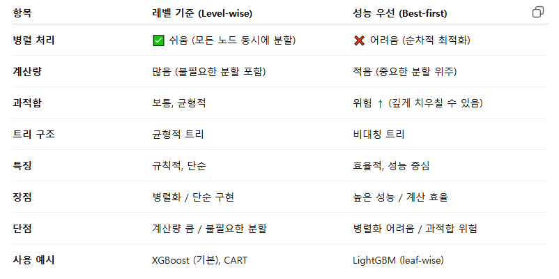
특징
- 규칙적 → 각 레벨 단위로 나눔
- 모든 후보 노드가 동시에 확장되므로 병렬 처리에 적합
- 불필요한 노드도 확장될 수 있음 → 계산량 낭비
장점
- 구현이 간단, GPU/분산 환경에서 효율적 (LightGBM 이전의 XGBoost 방식)
- 병렬 처리 가능.
단점
- 모든 노드를 일괄적으로 확장 → 계산량이 커짐.
- 상대적으로 과적합 위험이 큼 (불필요한 분할 포함).
- 트리의 "중요한 경로"가 빠르게 성장하지 못함.
- 비효율적인 분할을 지닐 가능성이 높음
성능 우선 성장 (Best-first / Leaf-wise)
- 모든 리프 후보 중 손실 감소(gain)가 가장 큰 노드부터 확장.
- 즉, 효율적인 분할만 우선적으로 성장시킴
특징
- 계산 자원을 성능이 좋은 분할에 집중.
- 비대칭 트리가 만들어질 수 있음 (깊은 쪽은 깊고, 다른 쪽은 얕음).
장점
- 적은 깊이에서도 높은 정확도 가능.
- 계산량이 상대적으로 절약됨 (효율적 분할 위주)
- LightGBM이 채택 → 빠른 학습, 좋은 성능.
단점
- 특정 분할에 너무 집중, 학습 데이터에 더 가깝게 맞춤 → 과적합 위험이 있음 (특히 작은 데이터셋)
- 병렬화 어려움 (순차적으로 최적 노드를 찾아야 하므로).
- 비대칭 트리 구조 → 해석성이 떨어질 수 있음.
- 노드 선택 과정에서 관리 비용이 추가

지니 불순도 vs 엔트로피
| 지니 불순도 | 엔트로피 | |
| 계산 비용 | 더 단순 (제곱 연산) | 로그 연산 포함 |
| 값의 범위 | 0 ~ 0.5 (이진), 0 ~ 1-1/K (다중) | 0 ~ log₂(K) |
| 최대치 시점 | 클래스 균등 분포일 때 | 클래스 균등 분포일 때 |
| 트리 분할 특성 | 다중 클래스를 고립 시키는 경향 | 더 균형 잡힌 트리 |
ㄴ 한 노드의 지니 불순도는 부모의 불순도보다 높은 경우가 발생할 수 있다. (AAABA -> AAA / BA)
ㄴ 0이면 순수한 값
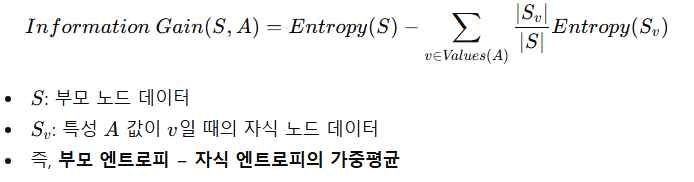
정보이득
- 특정 특성(Feature)으로 분할했을 때 엔트로피가 얼마나 줄어드는지를 측정
- 불순도가 얼마나 감소했는지(개선 효과) 측정 → 정보이득이 클수록 좋은 분할
- 결정트리는 정보이득이 가장 큰 feature를 분할 기준으로 선택
정보이득 계산
- 부모 노드 엔트로피 = 0.94
- 특정 feature로 분할했더니 자식 2개 엔트로피 가중평균 = 0.50이라면
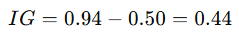
→ 정보이득 0.44 → 엔트로피가 많이 줄었으므로 좋은 분할
예시
- 10개의 부모 노드에 대해 positive 6 + negative 4인 경우
- 부모 노드의 엔트로피는 0.442 + 0.528 = 0.97

- feature A로 다음과 같이 분할 했다면
→ 자식 노드 Left (p 4 / n 1)

→ 자식 노드 Right (p 2 / n 3)

자식 노드의 가중 평균은 다음과 같다.

이때, 정보이득은 다음과 같다.
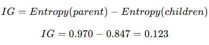
엔트로피가 0.123만큼 감소하게 되므로 어느 정도 좋은 분할이라고 할 수 있다.
트리의 특성 중요도 (feature_importances_)
- 총 합은 1
- 항상 양수
- 어떤 클래스를 지지하는지는 알 수 없음.
의사결정나무 알고리즘
ID3 (Iterative Dichotomiser 3)
- 가장 초기의 의사결정나무 알고리즘
- 정보이득(Information Gain)을 사용해 분할 기준을 선택
- 엔트로피(Entropy)를 기반으로 계산
- 속성 값이 많은 변수를 선호 (편향)
- 사용 지표 : 엔트로피(Entropy), 정보 이득(Information Gain)
CART (Classification and Regression Tree)
- 가장 널리 쓰이는 알고리즘 (sklearn의 DecisionTreeClassifier/Regressor가 이 방식)
- 분류 : 지니 불순도(Gini Impurity), 엔트로피 (옵션) 사용
- 회귀 : MSE(Mean Squared Error) 또는 MAE 사용
- 이진 분할만 허용 (Binary Split)
- 입력변수들의 선형결합들 중에서 최적의 분리를 찾는다.
C4.5, C5.0
- ID3의 개선 버전, 실무에서 많이 사용되던 알고리즘
- 정보이득비율(Gain Ratio) 사용 → 값이 많은 변수 선호하는 문제 해결
- 연속형 변수도 처리
- 가지치기(pruning) 포함
- 다지 분할 허용, 범주형 입력변수는 범주의 수만큼 분리가 일어난다.
- 사용 지표 : 엔트로피(Entropy), 정보이득비율(Gain Ratio)
CHAID (Chi-square Automatic Interaction Detection)
- 카이제곱 검정(Chi-square test)을 이용해 분할
- 다지 분할(Multi-way split) 가능
- 대규모 범주형 데이터에 자주 사용
- 사용 지표 : 카이제곱 통계량(Chi-square), F-test, Likelihood Ratio
QUEST (Quick, Unbiased, Efficient Statistical Tree)
- 분할 기준 선택 편향이 적도록 설계된 알고리즘
- 연속형, 범주형 데이터 모두 효율적으로 처리
하이퍼 파라미터
from sklearn.tree import DecisionTreeClassifier, DecisionTreeRegressor

DecisionTreeClassifier(
    criterion='gini',
    splitter='best',
    max_depth=None,
    min_samples_split=2,
    min_samples_leaf=1,
    min_weight_fraction_leaf=0.0,
    max_features=None,
    random_state=None,
    max_leaf_nodes=None,
    min_impurity_decrease=0.0,
    min_impurity_split=None,
    class_weight=None, # Classifier에만 존재
    presort=False,
)

DecisionTreeRegressor(
    criterion='mse',
    splitter='best',
    max_depth=None,
    min_samples_split=2,
    min_samples_leaf=1,
    min_weight_fraction_leaf=0.0,
    max_features=None,
    random_state=None,
    max_leaf_nodes=None,
    min_impurity_decrease=0.0,
    min_impurity_split=None,
    presort=False,
)
criterion
- gini : 지니 불순도
- entropy : 정보 이득(information gain)
- mse : 평균제곱오차(mean squared error), 특징 선택 기준으로서 분산 감소(variance reduction) 와 동일
또한 각 말단 노드(의 평균을 사용하여 L2 손실을 최소화합니다.
- friedman_mse : 평균제곱오차(MSE)를 사용하지만, 잠재적 분할에 대해 Friedman의 개선 점수를 함께 적용
- mae : 평균절대오차(mean absolute error), 각 말단 노드의 중앙값을 사용하여 L1 손실을 최소화
splitter
- best : 가장 좋은(최적) 분할 선택
- random : 무작위 후보 중 가장 좋은 분할 선택
max_depth
- 모든 leaf가 순수해질 때까지, 혹은 leaf 내 샘플 수가 min_samples_split 보다 작아질 때까지 노드를 계속 확장
import matplotlib.pyplot as plt
from sklearn.tree import DecisionTreeClassifier, plot_tree
from sklearn.datasets import make_moons
# create dataset
X, y = make_moons(n_samples=300, noise=0.25, random_state=42)
# models
model2 = DecisionTreeClassifier(max_depth=2, random_state=42)
model5 = DecisionTreeClassifier(max_depth=5, random_state=42)
model2.fit(X, y)
model5.fit(X, y)
# plot the trees
plt.figure(figsize=(12, 6))
plot_tree(model2, filled=True)
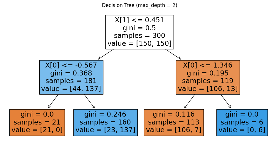
plt.title("Decision Tree (max_depth = 2)")
plt.show()
plt.figure(figsize=(18, 10))
plot_tree(model5, filled=True)
plt.title("Decision Tree (max_depth = 5)")
plt.show()
max_depth = 2 vs 5

* 참고
(DecisionTree 모델).apply(Data)로 어떤 노드에 도달했는지 알 수 있다.
model2.apply(X)

```
array([3, 3, 3, 3, 3, 3, 3, 5, 3, 3, 3, 5, 3, 5, 3, 3, 3, 3, 2, 3, 5, 2,
       ..., dtype=int64)
```
np.unique로 도달한 node 번호를 count하면 위의 그림의 samples와 개수가 일치한다.
import numpy as np

value, count = np.unique(model2.apply(X), return_counts=True)
value, count

# (array([2, 3, 5, 6], dtype=int64), array([ 21, 160, 113,   6], dtype=int64))
min_samples_split
- int → 그 값을 최소 샘플 수로 사용
- float → 전체 샘플 수 대비 비율이며, ceil(min_samples_split * n_samples) 개 이상 필요
- 한 내부 노드(node) 를 분할(더 쪼개기)하려면 그 노드에 최소 이만큼의 샘플이 있어야 한다는 제한
- 노드에 샘플이 너무 적을 때 분할을 허용하면 아주 작은 서브트리가 생기고 과적합이 발생하기 쉬움
- "아주 작은 그룹에서 분할하지 마라"는 제한 → 현재 노드의 샘플 수가 min_samples_split 미만이면 분할 X
ex. 데이터셋 전체 샘플 수가 10이고, 어떤 노드가 현재 3개의 샘플을 갖고 있다면?
- min_samples_split=4 이면 분할 불가 (3 < 4)
- min_samples_split=3 이면 분할 가능 (3 ≥ 3)
- min_samples_split=2 이면 분할 가능 (3 ≥ 2)
import matplotlib.pyplot as plt
from sklearn.tree import DecisionTreeClassifier, plot_tree
from sklearn.datasets import make_moons

# create dataset
X, y = make_moons(n_samples=300, noise=0.25, random_state=42)

# models with different min_samples_split
model0 = DecisionTreeClassifier(min_samples_split=113, random_state=42)
model1 = DecisionTreeClassifier(min_samples_split=114, random_state=42)

model0.fit(X, y)
model1.fit(X, y)

# plot the trees
plt.figure(figsize=(14, 8))
plot_tree(model0, filled=True)
plt.title("Decision Tree (min_samples_split = 113)")
plt.show()

plt.figure(figsize=(14, 8))
plot_tree(model1, filled=True)
plt.title("Decision Tree (min_samples_split = 114)")
plt.show()
min_samples_split = 113 vs 114
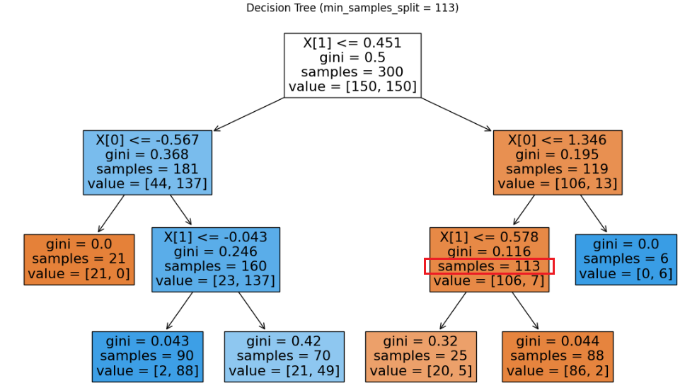
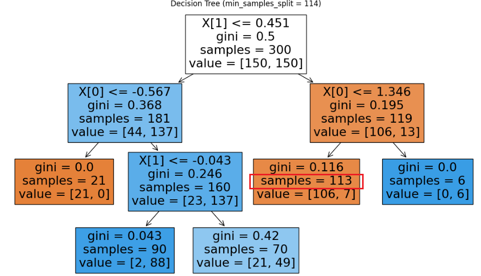
samples가 113인 경우
- min_samples_split=113 : 113은 min_samples_split 미만이 아니므로 분할 가능
- min_samples_split=114 : 113는 min_samples_split 미만이므로 분할 불가
min_samples_leaf
- 분할 후 왼쪽 / 오른쪽 모두 최소 min_samples_leaf 개 이상이어야 해당 split 후보가 유효.
- int → 해당 숫자를 사용
- float → 전체 샘플 수 대비 비율로 처리 ceil(min_samples_leaf * n_samples) 적용
- 회귀의 경우 모델이 부드러워지는 효과가 있음
ㄴ 트리가 너무 잘게 쪼개져서 지그재그 같은 불연속적인 예측을 하지 않는다.
- 각 리프(leaf) 에 남아 있어야 하는 최소 샘플 수를 지정
- 자식 노드(분할 후의 두 쪽)에 너무 작은 리프가 생기는 것을 막는다.
- 어떤 분할은 min_samples_split 조건을 만족해도, 자식 중 하나가 min_samples_leaf 미만이면 분할 불가
ex. 전체 10개 샘플, 루트에서 가능한 분할이 (왼쪽 1, 오른쪽 9)라면?
- min_samples_split=2(허용) 이라도 min_samples_leaf=2이면 해당 분할은 거부된다 (왼쪽이 1 < 2)
import matplotlib.pyplot as plt
from sklearn.tree import DecisionTreeClassifier, plot_tree
from sklearn.datasets import make_moons

# create dataset
X, y = make_moons(n_samples=300, noise=0.25, random_state=42)

# models with different min_samples_leaf
model0 = DecisionTreeClassifier(min_samples_leaf=59, random_state=42)
model1 = DecisionTreeClassifier(min_samples_leaf=60, random_state=42)

model0.fit(X, y)
model1.fit(X, y)

# plot the trees
plt.figure(figsize=(14, 8))
plot_tree(model0, filled=True)
plt.title("Decision Tree (min_samples_leaf = 59)")
plt.show()

plt.figure(figsize=(14, 8))
plot_tree(model1, filled=True)
plt.title("Decision Tree (min_samples_leaf = 60)")
plt.show()
min_samples_leaf = 59 vs 60
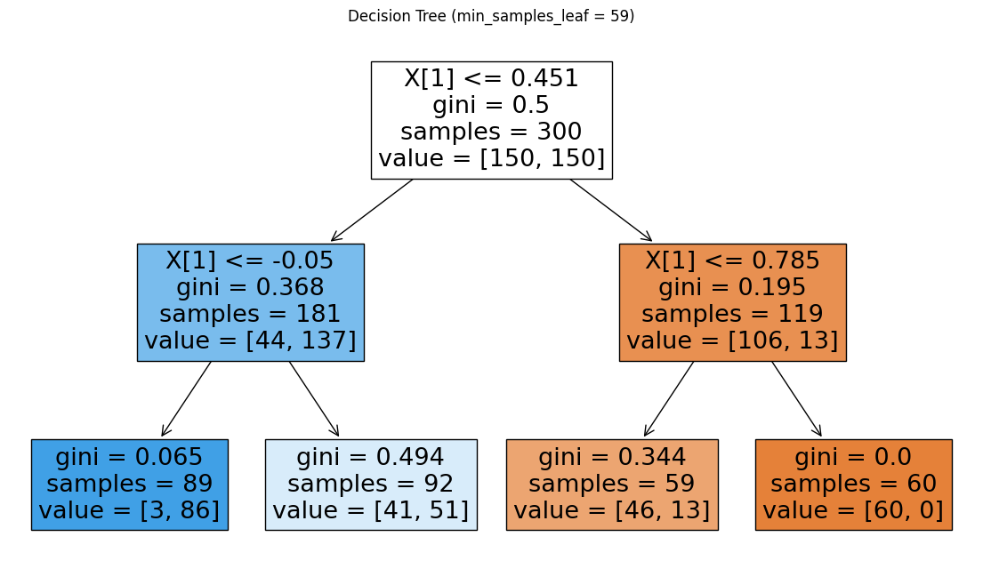
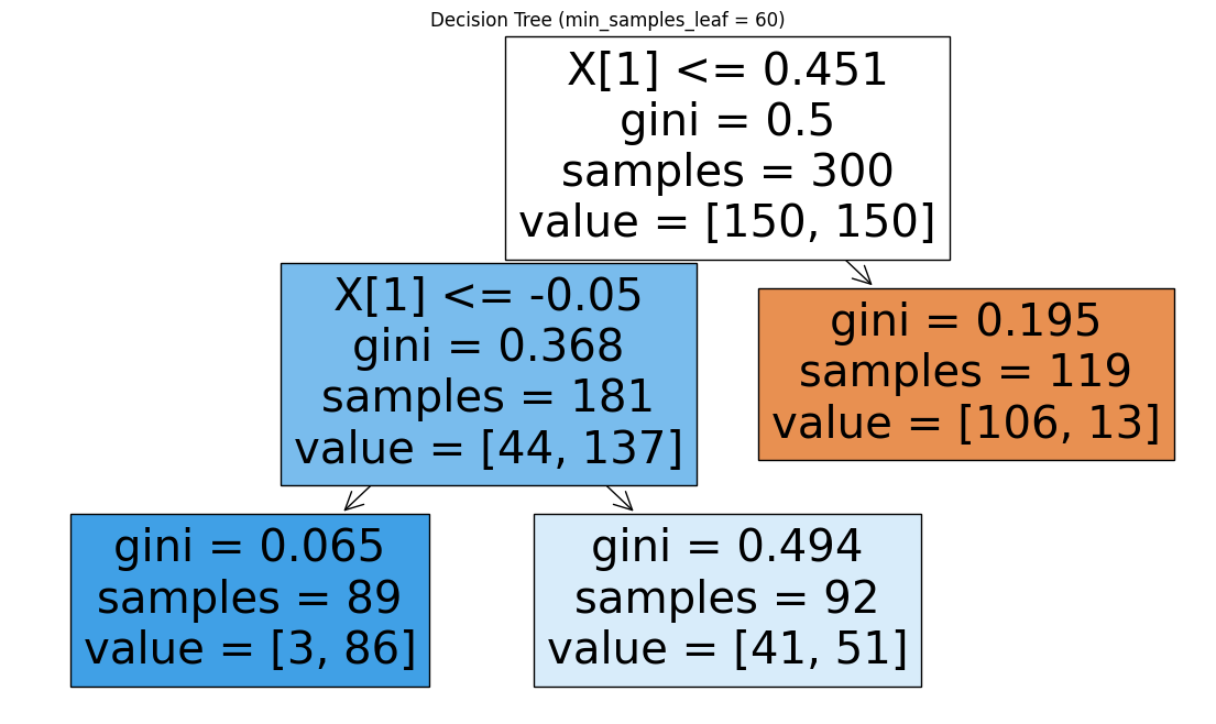
min_samples_leaf가 59인 경우는 오른쪽 노드가 분할 가능하지만, 60인 경우는 분할이 불가능하다. (119 = 59 + 60)
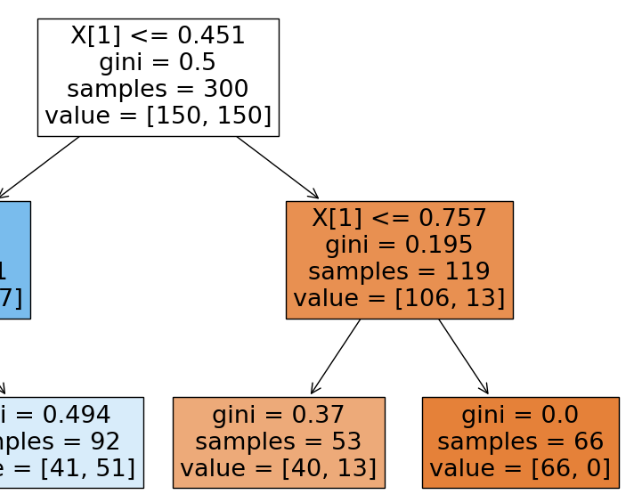
또한 min_samples_leaf를 50으로 설정했을 때, 오른쪽 노드는 66개(gini = 0)로 분류가 끝났지만
min_samples_leaf를 59로 높이면 오른쪽 노드의 분류 60개로 적어진다.
min_weight_fraction_leaf
- sample_weight 를 제공하지 않으면 모든 샘플 가중치는 동일
import matplotlib.pyplot as plt
from sklearn.tree import DecisionTreeClassifier, plot_tree
from sklearn.datasets import make_moons

# create dataset
X, y = make_moons(n_samples=300, noise=0.25, random_state=42)

# models with min_weight_fraction_leaf
# 0.20 ≈ 60/300
model0 = DecisionTreeClassifier(random_state=42)
model1 = DecisionTreeClassifier(min_weight_fraction_leaf=0.20, random_state=42)

model0.fit(X, y)
model1.fit(X, y)

# plot the trees
plt.figure(figsize=(14, 8))
plot_tree(model0, filled=True)
plt.title("Decision Tree (min_weight_fraction_leaf = 0.0)")
plt.show()

plt.figure(figsize=(14, 8))
plot_tree(model1, filled=True)
plt.title("Decision Tree (min_weight_fraction_leaf = 0.20)")
plt.show()
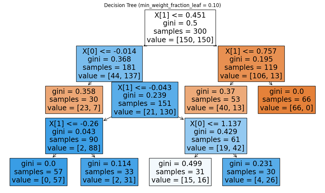
min_weight_fraction_leaf = 0.0 vs 0.2
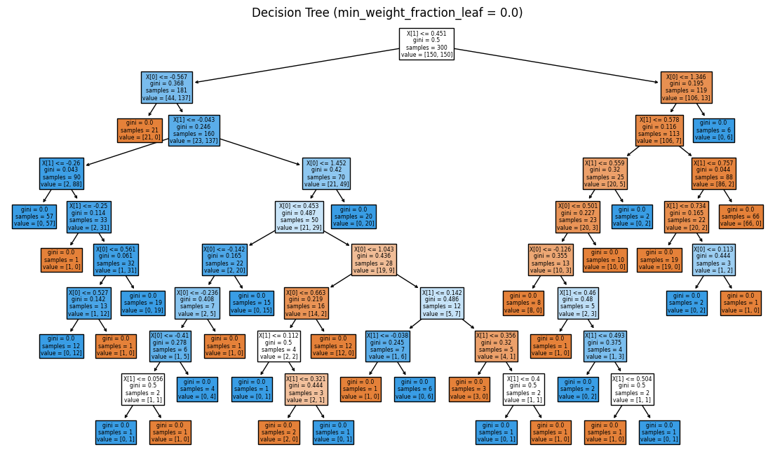
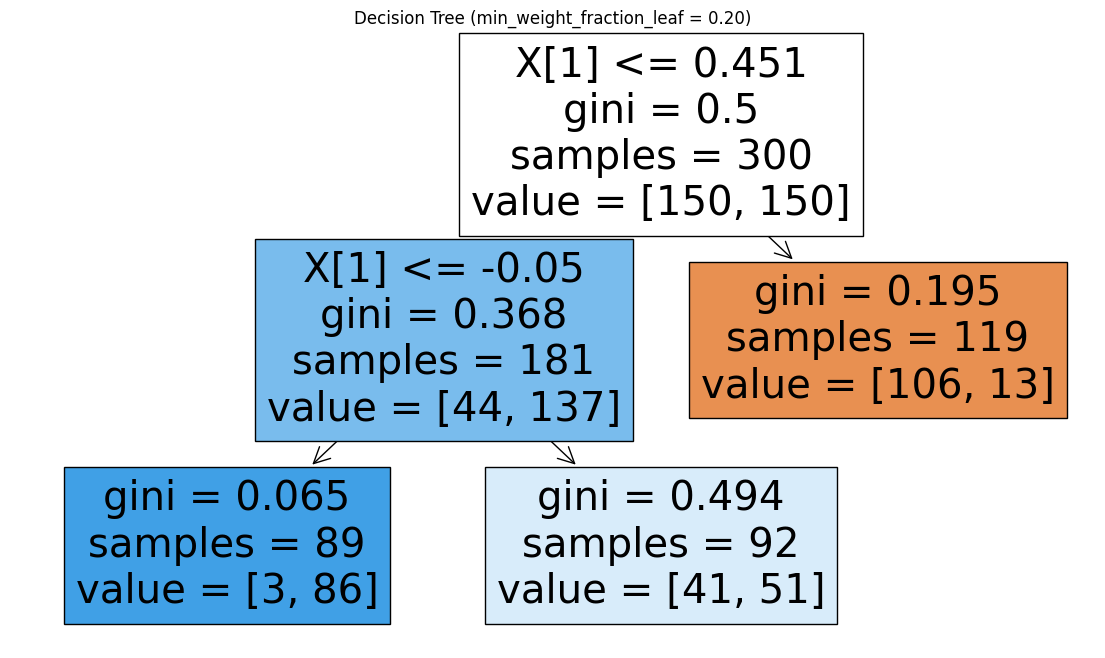
전체 샘플이 300개
→ min_weight_fraction_leaf=0.2라면, 리프 노드는 전체 샘플 수의 20% 이상을 가져야 한다.
0.1로 낮출 경우, 모든 리프 노드가 전체 샘플 수의 10% 이상(30개)을 가지는 것을 알 수 있다.
max_features
- int → 해당 개수의 feature 사용
- float → 비율이며 int(max_features * n_features) 사용
- auto → sqrt(n_features)
- sqrt → sqrt(n_features)
- log2 → log2(n_features)
- None → 모든 feature 사용
- 분할을 찾을 때 최소한 한 개의 유효한 분할을 찾을 때까지 계속 시도
- 노드마다 무작위로 선택된 feature subset을 보고 최적의 분할을 찾는다.
→ 같은 트리 내에서도 각 노드마다 선택되는 feature가 다를 수 있음
- 실제로는 max_features 보다 더 많이 확인될 수도 있음.
- max_features를 줄일수록 트리가 덜 깊고 덜 세밀한 구조, 과적합 감소
max_leaf_nodes
- None → 제한 없음
- 트리에서 허용할 리프(잎) 노드의 최대 개수를 지정
ㄴ 최종 리프(terminal) 노드의 최대 개수를 제한하는 옵션
- max_leaf_nodes가 주어지면 best-first(가장 불순도 감소가 큰 노드부터 분할) 방식으로 트리를 확장
- 전체 불순도 감소량이 가장 큰 분할을 우선해서 선택하여 리프 수가 max_leaf_nodes가 될 때까지 분할을 진행
ㄴ 가장 이득(불순도 감소)이 큰 분할들만 골라서 리프 수를 만듬
import matplotlib.pyplot as plt
from sklearn.tree import DecisionTreeClassifier, plot_tree
from sklearn.datasets import make_moons

# create dataset
X, y = make_moons(n_samples=300, noise=0.25, random_state=42)

# models with different max_leaf_nodes
model0 = DecisionTreeClassifier(max_leaf_nodes=3, random_state=42)
model1 = DecisionTreeClassifier(max_leaf_nodes=7, random_state=42)

model0.fit(X, y)
model1.fit(X, y)

# plot the trees
plt.figure(figsize=(14, 8))
plot_tree(model0, filled=True)
plt.title("Decision Tree (max_leaf_nodes = 3)")
plt.show()

plt.figure(figsize=(14, 8))
plot_tree(model1, filled=True)
plt.title("Decision Tree (max_leaf_nodes = 7)")
plt.show()
max_leaf_nodes = 3 vs 7


최종 리프(terminal) 노드가 각가 3개 / 7개
min_impurity_decrease
- float (default=0.)
- weight 기반 계산식
- 노드를 분할할 최소 impurity 감소 기준
- 트리는 어떤 노드를 나눌 때, 분할로 얻는 impurity 감소량 ≥ min_impurity_decrease 인 경우에만 분할을 허용
- 이 값이 커질수록 분할 조건이 엄격해짐 → 트리가 덜 깊어짐 → 과적합 방지
N_t / N * (impurity - N_t_R / N_t * right_impurity - N_t_L / N_t * left_impurity)
import matplotlib.pyplot as plt
from sklearn.tree import DecisionTreeClassifier, plot_tree
from sklearn.datasets import make_moons

# create dataset
X, y = make_moons(n_samples=300, noise=0.25, random_state=42)

# models with different min_impurity_decrease
model0 = DecisionTreeClassifier(min_impurity_decrease=0.01, random_state=42)
model1 = DecisionTreeClassifier(min_impurity_decrease=0.03, random_state=42)

model0.fit(X, y)
model1.fit(X, y)

# plot the trees
plt.figure(figsize=(14, 8))
plot_tree(model0, filled=True)
plt.title("Decision Tree (min_impurity_decrease = 0.01)")
plt.show()

plt.figure(figsize=(14, 8))
plot_tree(model1, filled=True)
plt.title("Decision Tree (min_impurity_decrease = 0.03)")
plt.show()
min_impurity_decrease = 0.01 vs 0.03


class_weight
- 주지 않으면 모든 클래스 동일 가중치
- 다중 output 의 경우 각 output별 dict 필요
- sample_weight가 있으면 두 가중치가 곱해짐.
class_weight = {0: 1, 1: 5}  # 클래스 1의 중요도를 5배로
clf = DecisionTreeClassifier(class_weight=class_weight)
- balanced 모드는 n_samples / (n_classes * np.bincount(y)) 비율로 자동 조정
- 이 경우 sklearn이 자동으로 클래스 빈도에 반비례하여 가중치를 계산

Attributes
    classes_ : array of shape = [n_classes] or a list of such arrays
        The classes labels (single output problem),
        or a list of arrays of class labels (multi-output problem).

    feature_importances_ : array of shape = [n_features]
        The feature importances. The higher, the more important the
        feature. The importance of a feature is computed as the (normalized)
        total reduction of the criterion brought by that feature.  It is also
        known as the Gini importance [4]_.

    max_features_ : int,
        The inferred value of max_features.

    n_classes_ : int or list
        The number of classes (for single output problems),
        or a list containing the number of classes for each
        output (for multi-output problems).

    n_features_ : int
        The number of features when ``fit`` is performed.

    n_outputs_ : int
        The number of outputs when ``fit`` is performed.

    tree_ : Tree object
        The underlying Tree object. Please refer to
        ``help(sklearn.tree._tree.Tree)`` for attributes of Tree object and
        :ref:`sphx_glr_auto_examples_tree_plot_unveil_tree_structure.py`
        for basic usage of these attributes.
classes_ : array or list of arrays
클래스 레이블들
feature_importances_ : array [n_features]
- 특성 중요도
- 지니 불순도 감소량 기준 normalized
max_features_ : int
- 실제로 사용된 max_features 값
n_classes_ : int or list
- 클래스 개수
n_features_ : int
- fit 시 feature 개수
n_outputs_ : int
- 출력 개수
tree_ : Tree 객체
- 실제 트리 구조
'개발 > Python' 카테고리의 다른 글
| LogisticRegression Hyper Parameters and Attributes (0) | 2025.09.14 |
|---|---|
| 카이제곱 검정 (0) | 2025.09.14 |
| 검정 통계량 T, 평균의 차이와 신뢰구간 (0) | 2025.09.08 |
| 병합적 군집분석 계산 방법 비교 (linkage) (0) | 2025.09.08 |
| XGBoost Hyper Parameters and Attributes (0) | 2025.09.08 |


댓글