LogisticRegression
- t-검정을 했을 때, 클래스 레이블 간에 유의미한 차이가 없다면 피처로 선택 X
- 로지스틱 회귀에서 독립 변수는 정규성 가정이 불필요
- 오차항에 대한 정규성 가정도 불필요
- 확률 범위를 출력할 때는 sigmoid 함수를 사용한다.
- 단일 로지스틱 회귀 모델은 다중 클래스 분류를 위해 소프트맥스(softmax) 함수를 사용한다.
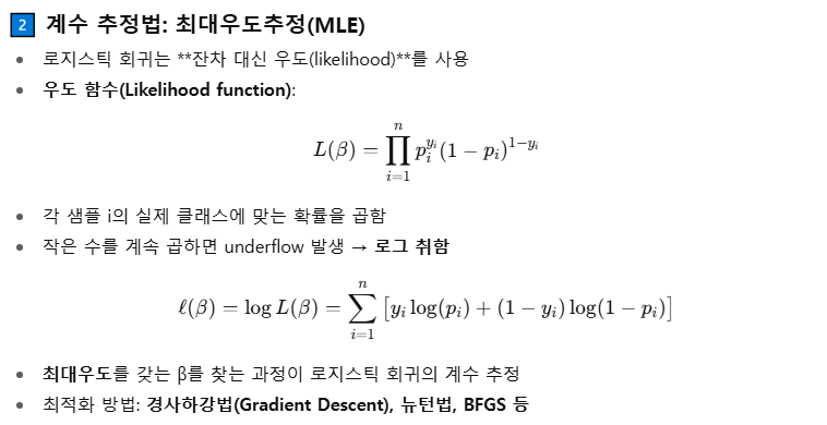
- 계수추정법 : 최대우도추정법 (로지스틱 회귀는 잔차대신 우도를 사용, y축 좌표 = 1일 확률 = 우도)
- 전체 모델의 적합도를 평가할 때 카이제곱 검정(Chi-square test) 사용
- 잔차대신 우도 기반 검정(Likelihood Ratio Test) 수행
- 경사하강법, Newton-Rapson 사용
- 고전적인 퍼셉트론(확률 추정 불가)에서 시그모이드 활성화 함수 + 경사 하강법을 사용하면 로지스틱 회귀와 동일
import numpy as np
import matplotlib.pyplot as plt
from PIL import Image
from io import BytesIO

def logistic(x, b0=0, b1=1):
    return 1 / (1 + np.exp(-(b0 + b1 * x)))

x = np.linspace(-5, 5, 300)

# --- β1 > 0 그래프 생성 ---
fig1 = plt.figure()
plt.plot(x, logistic(x, b1=2))
plt.title("β1 > 0")
plt.xlabel("x")
plt.ylabel("Probability")
plt.grid(True)

buf1 = BytesIO()
plt.savefig(buf1, format="png", bbox_inches="tight")
plt.close(fig1)
buf1.seek(0)
img1 = Image.open(buf1)

# --- β1 < 0 그래프 생성 ---
fig2 = plt.figure()
plt.plot(x, logistic(x, b1=-2))
plt.title("β1 < 0")
plt.xlabel("x")
plt.ylabel("Probability")
plt.grid(True)

buf2 = BytesIO()
plt.savefig(buf2, format="png", bbox_inches="tight")
plt.close(fig2)
buf2.seek(0)
img2 = Image.open(buf2)

# --- 두 이미지를 좌우로 합치기 ---
w1, h1 = img1.size
w2, h2 = img2.size

combined = Image.new("RGB", (w1 + w2, max(h1, h2)), (255, 255, 255))
combined.paste(img1, (0, 0))
combined.paste(img2, (w1, 0))

combined
하이퍼 파라미터
from sklearn.linear_model import LogisticRegression

LogisticRegression(
    penalty='l2',
    dual=False,
    tol=0.0001,
    C=1.0,
    fit_intercept=True,
    intercept_scaling=1,
    class_weight=None,
    random_state=None,
    solver='warn',
    max_iter=100,
    multi_class='warn',
    verbose=0,
    warm_start=False,
    n_jobs=None,
    l1_ratio=None,
)
penalty
- str, 'l1', 'l2', 'elasticnet' 또는 'none', 기본값='l2'
- 페널티에 사용할 규제(norm)를 지정
- 'newton-cg', 'sag', 'lbfgs' 솔버는 L2 페널티만 지원
- 'elasticnet'은 'saga' 솔버에서만 지원
- 'none'으로 설정하면(단, liblinear 솔버는 지원하지 않음) 정규화를 적용 X
로지스틱 회귀의 로그 손실


L1 정규화

L2 정규화

Elastic-Net 정규화

α = 1 → L1 정규화
α = 0 → L2 정규화
dual : bool
- Dual 또는 primal formulation 사용 여부
- 최적화 문제를 풀 때 "원래 문제(primal)" 대신 쌍대 문제(dual)를 풀 것인지를 결정
- Dual formulation은 liblinear 솔버의 L2 페널티에서만 구현
- n_samples > n_features인 경우 dual=False를 권장 (특징 수가 많을 때 효율적인 옵션)

tol : float
- 최적화 종료 조건 허용 오차(tolerance).
- 로지스틱 회귀는 가중치 를 반복(iterative)으로 업데이트하며 최적화
- 반복 과정에서 손실 함수나 가중치 변화가 충분히 작아지면 멈추는 기준

C : float (양수)
- 정규화 강도의 역수
- SVM과 유사하게, 값이 작을수록 강한 정규화를 의미
- C가 작을수록 규제가 강해져 모델이 단순해짐.

↓

intercept_scaling : float
- 주로 liblinear + L1 / L2 + fit_intercept=True일 때만 의미 있음
- liblinear solver에서 사용되는 가상의 특성(synthetic feature)의 스케일을 조절하는 값
- 이 경우 x는 [x, intercept_scaling]이 되어 "합성(synthetic) 특성"이 인스턴스 벡터에 추가
- intercept는 (intercept_scaling * 합성 특성 가중치)로 계산
- 참고 : 합성 특성 가중치도 L1/L2 정규화가 적용
- 정규화 영향을 줄이려면 intercept_scaling 값을 증가
L1 / L2 정규화를 적용하면 절편에도 규제가 걸림
→ 작은 값이면 정규화로 인해 절편이 너무 작아질 수 있음 → 결정 경계 이동 문제
→ intercept_scaling을 키우면, 절편에 대한 정규화 영향이 상대적으로 작아짐
class_weight
- dict 또는 'balanced', 기본값=None
- 클래스별 가중치를 {class_label: weight} 형식으로 지정.
- 지정하지 않으면 모든 클래스 가중치는 1로 처리
- sample_weight이 지정되면 곱해진다.
- 'balanced' 모드는 y 값의 클래스 빈도에 반비례하도록 자동으로 가중치를 조정

또는 딕셔너리로 지정
cw = {0:0.1, 1:5.0} # 클래스 1의 중요도가 5.0 / 0.1 = 50배 더 크게 보는 설정
clf2 = LogisticRegression(class_weight=cw).fit(X, y)
solver : str
- {'newton-cg', 'lbfgs', 'liblinear', 'sag', 'saga'}, 기본값='liblinear'
- 작은 데이터셋: 'liblinear' 권장
- 큰 데이터셋: 'sag', 'saga' 빠름
- 다중 클래스: 'newton-cg', 'sag', 'saga', 'lbfgs'는 multinomial 지원, 'liblinear'는 OvR만 가능
- 'newton-cg', 'lbfgs', 'sag', 'saga': L2 또는 정규화 없음
- 'liblinear', 'saga': L1 가능
- 'saga': elasticnet 가능
- 'liblinear': no penalty 불가
- 참고: 'sag', 'saga'는 특성 스케일이 비슷해야 빠른 수렴 보장.
| Solver | 설명 | 지원 패널티 | 장점 / 특징 |
| liblinear | 라이브러리 LIBLINEAR 기반, 이진/작은 데이터에 적합 |
L1, L2 | 작은 데이터셋, OVR(One-vs-Rest) 멀티클래스 지원 |
| newton-cg | 뉴턴 방법 기반 | L2 | 다중 클래스, 안정적 수렴 큰 데이터보다는 중간 크기 데이터 |
| lbfgs | L-BFGS (Quasi-Newton) | L2 | 다중 클래스, 메모리 효율적 중간/큰 데이터 적합 |
| sag | Stochastic Average Gradient | L2 | 큰 데이터, 빠른 수렴 특징 스케일 조정 필요 |
| saga | SAG 변형, Elastic-Net 지원 | All | 큰 데이터, 희소 행렬 Elastic-Net 지원, L1 포함 |
max_iter : int
- 솔버 수렴을 위한 최대 반복 횟수
multi_class : str
- {'ovr', 'multinomial', 'auto'}, 기본값='ovr'
- 'ovr': 각 라벨에 대해 이진 문제를 학습
- 'multinomial': 전체 확률 분포에 대해 multinomial loss 최소화
- 'auto': 데이터가 이진이거나 solver='liblinear'이면 'ovr', 아니면 'multinomial'
l1_ratio : float
- Elastic-Net 혼합 파라미터 (0 <= l1_ratio <= 1)
- penalty='elasticnet'일 때만 사용.
Attributes
    classes_ : array, shape (n_classes, )
        A list of class labels known to the classifier.

    coef_ : array, shape (1, n_features) or (n_classes, n_features)
        Coefficient of the features in the decision function.

        `coef_` is of shape (1, n_features) when the given problem is binary.
        In particular, when `multi_class='multinomial'`, `coef_` corresponds
        to outcome 1 (True) and `-coef_` corresponds to outcome 0 (False).

    intercept_ : array, shape (1,) or (n_classes,)
        Intercept (a.k.a. bias) added to the decision function.

        If `fit_intercept` is set to False, the intercept is set to zero.
        `intercept_` is of shape (1,) when the given problem is binary.
        In particular, when `multi_class='multinomial'`, `intercept_`
        corresponds to outcome 1 (True) and `-intercept_` corresponds to
        outcome 0 (False).

    n_iter_ : array, shape (n_classes,) or (1, )
        Actual number of iterations for all classes. If binary or multinomial,
        it returns only 1 element. For liblinear solver, only the maximum
        number of iteration across all classes is given.

        .. versionchanged:: 0.20

            In SciPy <= 1.0.0 the number of lbfgs iterations may exceed
            ``max_iter``. ``n_iter_`` will now report at most ``max_iter``.
classes_
- 클래스 레이블들
coef_
- 결정 함수(feature) 계수
- 이진 문제: shape=(1, n_features)
- multi_class='multinomial': outcome 1(True)=coef_, outcome 0(False)=-coef_
intercept_
- 결정 함수에 더해지는 상수항
- fit_intercept=False이면 0
n_iter_
- 실제 반복 횟수. binary/multinomial이면 1개 반환. liblinear는 최대 반복 횟수 반환
오즈와 오즈비


오즈비 예시
model = LogisticRegression(multi_class='ovr', solver='liblinear', C=1.0)
...
odds_ratios = np.exp(model.coef_) # 오즈비
로그 우도
- 모델이 데이터를 얼마나 잘 설명하는지 측정하는 지표

import numpy as np
from sklearn.linear_model import LogisticRegression
from sklearn.datasets import make_classification

# 데이터 생성
X, y = make_classification(n_samples=100, n_features=2, random_state=0)
clf = LogisticRegression().fit(X, y)

# 예측 확률
p = clf.predict_proba(X)[:, 1]

# 로그 우도
log_likelihood = np.sum(y * np.log(p) + (1 - y) * np.log(1 - p))
print("Log-likelihood:", log_likelihood)
잔차 이탈도 (Deviance)
- 잔차 이탈도는 로그 우도와 비교하여 모델 적합도를 평가하는 지표

deviance = -2 * log_likelihood
statsmodels의 logit에서는 로그 우도를 제공한다.
from statsmodels.formula.api import logit

...

model = logit('y ~ X1 + X2', df).fit()

np.exp(model.params) # 오즈비
model.llf # 로그 우도
model.llf * -2 # 잔차 이탈도'개발 > Python' 카테고리의 다른 글
| T 검정 (0) | 2025.09.14 |
|---|---|
| datetime (0) | 2025.09.14 |
| 카이제곱 검정 (0) | 2025.09.14 |
| DecisionTree Hyper Parameters and Attributes (0) | 2025.09.08 |
| 검정 통계량 T, 평균의 차이와 신뢰구간 (0) | 2025.09.08 |

댓글