XGBoost
- Gradient Boosting 기반(+ 최적화와 정규화)의 결정 트리 앙상블 알고리즘
- 여러 개의 약한 결정 트리(weak learners)를 순차적으로 학습시켜 오류를 점점 줄이는 방식
- 병렬 처리 가능 → 학습 속도 빠름
- 과적합 방지를 위한 정규화 기능 포함
- 결측치 처리 가능, 다양한 평가 지표 지원
- 대규모 데이터 처리에도 효율적
장점
- 높은 정확도
- 결측치 자동 처리
- 빠른 학습과 예측
- 과적합 방지 기능 내장
단점
- 모델 해석이 어려움
- 매우 큰 데이터셋에서는 메모리 사용량 증가
- 하이퍼 파라미터 튜닝이 필요
하이퍼 파라미터
from xgboost import XGBClassifier, XGBRegressor

XGBClassifier(
    max_depth=3,
    learning_rate=0.1,
    n_estimators=100,
    silent=True,
    objective='binary:logistic',
    booster='gbtree',
    n_jobs=1,
    nthread=None,
    gamma=0,
    min_child_weight=1,
    max_delta_step=0,
    subsample=1,
    colsample_bytree=1,
    colsample_bylevel=1,
    reg_alpha=0,
    reg_lambda=1,
    scale_pos_weight=1,
    base_score=0.5,
    random_state=0,
    seed=None,
    missing=None,
    **kwargs,
)

XGBRegressor(
    max_depth=3,
    learning_rate=0.1,
    n_estimators=100,
    silent=True,
    objective='reg:linear',
    booster='gbtree',
    n_jobs=1,
    nthread=None,
    gamma=0,
    min_child_weight=1,
    max_delta_step=0,
    subsample=1,
    colsample_bytree=1,
    colsample_bylevel=1,
    reg_alpha=0,
    reg_lambda=1,
    scale_pos_weight=1,
    base_score=0.5,
    random_state=0,
    seed=None,
    missing=None,
    **kwargs,
)
max_depth
- 기본 학습기의 최대 트리 깊이
- 결정트리와 동일
import numpy as np
import matplotlib.pyplot as plt
from sklearn.datasets import make_moons
from xgboost import XGBClassifier
from matplotlib.colors import ListedColormap

# 2차원 예제 데이터 생성
X, y = make_moons(n_samples=300, noise=0.25, random_state=42)

models = {
    "max_depth=2": XGBClassifier(max_depth=2, n_estimators=50, use_label_encoder=False, eval_metric='logloss'),
    "max_depth=10": XGBClassifier(max_depth=10, n_estimators=50, use_label_encoder=False, eval_metric='logloss')
}

# 결정 경계 시각화 함수
def plot_decision_boundary(model, X, y, ax, title):
    model.fit(X, y)
    x_min, x_max = X[:, 0].min() - 0.5, X[:, 0].max() + 0.5
    y_min, y_max = X[:, 1].min() - 0.5, X[:, 1].max() + 0.5
    xx, yy = np.meshgrid(np.linspace(x_min, x_max, 300),
                         np.linspace(y_min, y_max, 300))
    Z = model.predict(np.c_[xx.ravel(), yy.ravel()]).reshape(xx.shape)

    cmap_light = ListedColormap(['#FFAAAA', '#AAAAFF'])
    cmap_bold = ListedColormap(['#FF0000', '#0000FF'])

    ax.contourf(xx, yy, Z, alpha=0.3, cmap=cmap_light)
    ax.scatter(X[:, 0], X[:, 1], c=y, cmap=cmap_bold, edgecolor='k', s=50)
    ax.set_title(title)

# 그림 그리기
fig, axes = plt.subplots(1, 2, figsize=(12, 5))
for ax, (title, model) in zip(axes, models.items()):
    plot_decision_boundary(model, X, y, ax, title)

plt.show()
learning_rate
- 부스팅 학습률(Boosting Learning Rate)을 조절하는 하이퍼파라미터
- 여러 개의 트리를 순차적으로 학습해서 오류를 줄여나가는 방식
- 각 단계에서 새로운 트리는 이전 트리들의 잔차(residual)를 학습
- 이때 새로 만든 트리가 학습 과정에서 얼마나 크게 기여할지를 조절하는 것이 eta (learning_rate)
- eta가 작을수록 한 트리가 모델에 기여하는 정도가 작아지고, 학습이 느려지지만 일반화 성능이 좋아질 가능성이 높음
- 일반적으로: 0.01 ~ 0.3 사이에서 조정
import numpy as np
import matplotlib.pyplot as plt
from sklearn.datasets import make_moons
from xgboost import XGBClassifier
from matplotlib.colors import ListedColormap

# 2차원 예제 데이터 생성
X, y = make_moons(n_samples=300, noise=0.25, random_state=42)

models = {
    "max_depth=2": XGBClassifier(max_depth=2, n_estimators=50, use_label_encoder=False, eval_metric='logloss'),
    "max_depth=10": XGBClassifier(max_depth=10, n_estimators=50, use_label_encoder=False, eval_metric='logloss')
}

# 결정 경계 시각화 함수
def plot_decision_boundary(model, X, y, ax, title):
    model.fit(X, y)
    x_min, x_max = X[:, 0].min() - 0.5, X[:, 0].max() + 0.5
    y_min, y_max = X[:, 1].min() - 0.5, X[:, 1].max() + 0.5
    xx, yy = np.meshgrid(np.linspace(x_min, x_max, 300),
                         np.linspace(y_min, y_max, 300))
    Z = model.predict(np.c_[xx.ravel(), yy.ravel()]).reshape(xx.shape)

    cmap_light = ListedColormap(['#FFAAAA', '#AAAAFF'])
    cmap_bold = ListedColormap(['#FF0000', '#0000FF'])

    ax.contourf(xx, yy, Z, alpha=0.3, cmap=cmap_light)
    ax.scatter(X[:, 0], X[:, 1], c=y, cmap=cmap_bold, edgecolor='k', s=50)
    ax.set_title(title)

# 그림 그리기
fig, axes = plt.subplots(1, 2, figsize=(12, 5))
for ax, (title, model) in zip(axes, models.items()):
    plot_decision_boundary(model, X, y, ax, title)

plt.show()
→ learning_rate가 작을수록 일반화 성능이 높다. (과적합 방지)
n_estimators
- 학습할 부스팅 트리 수
objective : str 또는 callable
- 학습 작업 및 대응 학습 목표 지정, 또는 사용자 정의 목적 함수
- 사용자 정의 함수일 경우, 아래 형식을 따른다.

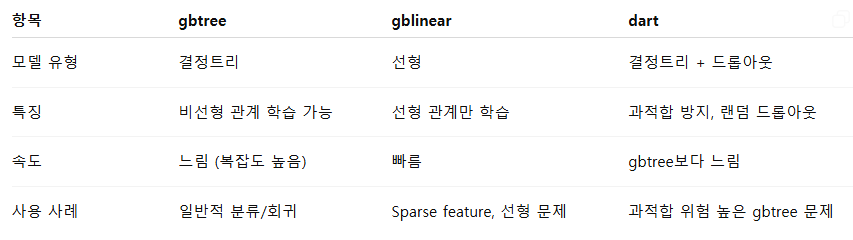
booster : str
- 사용할 부스터 유형 지정: 'gbtree', 'gblinear', 'dart'

gamma : float
- 리프 노드에서 추가 분할을 수행하기 위한 최소 손실 감소
- gamma가 클수록 분할 조건이 엄격해지고, 트리가 덜 깊고 단순하다.
- gamma = 0 → 작은 이득도 분할 허용 → 트리 복잡도 ↑
- 0 ~ 5 정도로 설정
import numpy as np
import matplotlib.pyplot as plt
from sklearn.datasets import make_moons
from xgboost import XGBClassifier

# 2차원 복잡한 데이터 (moons)
X, y = make_moons(n_samples=500, noise=0.3, random_state=42)

# gamma 값 리스트
gamma_values = [0, 5, 30]

# meshgrid 준비
x_min, x_max = X[:, 0].min() - 0.5, X[:, 0].max() + 0.5
y_min, y_max = X[:, 1].min() - 0.5, X[:, 1].max() + 0.5
xx, yy = np.meshgrid(np.arange(x_min, x_max, 0.01),
                     np.arange(y_min, y_max, 0.01))

plt.figure(figsize=(18,5))

for i, gamma_val in enumerate(gamma_values):
    # 모델 학습
    clf = XGBClassifier(n_estimators=50, max_depth=3, gamma=gamma_val,
                        use_label_encoder=False, eval_metric='logloss')
    clf.fit(X, y)

    # 결정 경계 계산
    Z = clf.predict(np.c_[xx.ravel(), yy.ravel()])
    Z = Z.reshape(xx.shape)

    # 그래프
    plt.subplot(1, 3, i+1)
    plt.contourf(xx, yy, Z, alpha=0.4, cmap=plt.cm.RdYlBu)
    plt.scatter(X[:,0], X[:,1], c=y, cmap=plt.cm.RdYlBu, edgecolor='k')
    plt.title(f'XGBoost Decision Boundary (gamma={gamma_val})')
    plt.xlabel('Feature 1')
    plt.ylabel('Feature 2')

plt.tight_layout()
plt.show()
→ gamma가 작을수록 과대적합되고 있는 것을 알 수 있다.
min_child_weight : int
- 자식 노드에서 필요한 최소 인스턴스 가중치 합계
- 트리의 자식 노드가 가지는 최소한의 샘플 가중치 합
- 이 값보다 작으면 해당 노드는 더 이상 분할되지 않음
- min_child_weight ↑ → 자식 노드 최소 샘플 수 증가 → 트리 단순화, 과적합 방지
- min_child_weight ↓ → 작은 노드도 분할 허용 → 트리 복잡, 과적합 가능
- 결정 트리의 min_samples_leaf / min_samples_split와 유사
- 1 ~ 10 사이에서 설정
import numpy as np
import matplotlib.pyplot as plt
from sklearn.datasets import make_moons
from xgboost import XGBClassifier

# 2차원 데이터 생성
X, y = make_moons(n_samples=500, noise=0.3, random_state=42)

# min_child_weight 값 리스트
child_weights = [1, 10, 20]

# meshgrid 준비
x_min, x_max = X[:, 0].min() - 0.5, X[:, 0].max() + 0.5
y_min, y_max = X[:, 1].min() - 0.5, X[:, 1].max() + 0.5
xx, yy = np.meshgrid(np.arange(x_min, x_max, 0.01),
                     np.arange(y_min, y_max, 0.01))

plt.figure(figsize=(18,5))

for i, weight in enumerate(child_weights):
    # 모델 학습
    clf = XGBClassifier(
        n_estimators=50,
        max_depth=3,
        min_child_weight=weight,
        use_label_encoder=False,
        eval_metric='logloss'
    )
    clf.fit(X, y)

    # 결정 경계 계산
    Z = clf.predict(np.c_[xx.ravel(), yy.ravel()])
    Z = Z.reshape(xx.shape)

    # 그래프
    plt.subplot(1, 3, i+1)
    plt.contourf(xx, yy, Z, alpha=0.4, cmap=plt.cm.RdYlBu)
    plt.scatter(X[:,0], X[:,1], c=y, cmap=plt.cm.RdYlBu, edgecolor='k')
    plt.title(f'XGBoost Decision Boundary (min_child_weight={weight})')
    plt.xlabel('Feature 1')
    plt.ylabel('Feature 2')

plt.tight_layout()
plt.show()
min_child_weight=1 → 작은 노드도 분할 → 결정 경계 세밀, 과적합 가능
min_child_weight=5 → 일부 작은 분할 억제 → 경계 조금 단순화
min_child_weight=20 → 작은 노드 거의 분할 안 함 → 경계 단순, 과적합 감소
→ min_child_weight가 작을수록 과대적합되고 있는 것을 알 수 있다.
max_delta_step : int
- 각 트리 가중치 추정 시 허용되는 최대 델타 스텝
- 각 leaf의 weight 최대 변화량 제한
- 한 단계에서 가중치가 너무 크게 변하지 않도록 안정화
- 학습이 너무 급격하게 진행되는 것을 방지
- 불균형/불안정 학습 안정화
- leaf output 변화 제한 ↑ → 학습 안정 ↑, 학습 속도 ↓
ex. 클래스 불균형 문제
- 작은 클래스의 gradient가 크면 학습이 불안정할 수 있음
- max_delta_step=1~10 정도 설정으로 안정화
subsample : float
- 학습 인스턴스의 샘플링 비율
- 값 범위 : 0 ~ 1
- 사용하는 데이터가 줄어들기 때문에 훈련 속도가 빨라짐
- 효과 : 과적합 방지, 일반화 향상
- 주의 : 너무 낮으면 학습 불안정, 너무 높으면 과적합
ex.
- subsample=0.6 → 트리 학습 시 데이터의 60%만 랜덤 선택
- 데이터 1000개, subsample=0.6
- 첫 번째 트리 학습 → 600개 샘플 사용
- 두 번째 트리 학습 → 또 다른 600개 샘플 랜덤 선택
colsample_bytree : float
- 각 트리를 구성할 때 컬럼 샘플링 비율
- 값 범위 : 0 ~ 1
- 각 트리를 학습할 때 전체 피처 중 일부만 사용
- 효과 : 과적합 방지, 랜덤성 증가
- 트리마다 선택되는 피처가 달라서 앙상블 다양성 증가
ex.
- 데이터 10개 피처, colsample_bytree=0.5
- 첫 번째 트리 → 10개 피처 중 5개만 선택
- 두 번째 트리 → 다른 5개 피처 선택 가능
colsample_bylevel : float
- 각 레벨의 분할에서 컬럼 샘플링 비율
- 값 범위 : 0 ~ 1
- 트리의 각 레벨(split)마다 사용할 피처 비율 조절
- 더 세밀한 샘플링으로 과적합 방지
- colsample_bytree와 함께 사용하면 트리 단위 + 레벨 단위 샘플링 가능
- 트리 내부에서 레벨별로 다른 피처를 허용 → 같은 트리 안에서도 다양한 구조를 만듦
- 고차원(특징 많은) 데이터에서 유용할 수 있음
import matplotlib.pyplot as plt
from sklearn.datasets import make_classification
from xgboost import XGBClassifier
import numpy as np

# Generate dataset
X, y = make_classification(
    n_samples=600,
    n_features=2,
    n_redundant=0,
    n_clusters_per_class=1,
    class_sep=1.2,
    random_state=0
)

# Grid
xx, yy = np.meshgrid(
    np.linspace(X[:, 0].min()-1, X[:, 0].max()+1, 300),
    np.linspace(X[:, 1].min()-1, X[:, 1].max()+1, 300)
)

col_vals0 = [1.0, 0.7, 0.5]
col_vals1 = [1.0, 0.7, 0.5]

plt.figure(figsize=(18, 12))

plot_idx = 1
for s in col_vals0:
    for c in col_vals1:
        model = XGBClassifier(
            colsample_bytree=s,
            colsample_bylevel=c,
            n_estimators=40,
            max_depth=3,
            learning_rate=0.1,
            use_label_encoder=False,
            eval_metric="logloss"
        )
        model.fit(X, y)

        Z = model.predict(np.c_[xx.ravel(), yy.ravel()])
        Z = Z.reshape(xx.shape)

        plt.subplot(len(sub_vals), len(col_vals), plot_idx)
        plt.contourf(xx, yy, Z, alpha=0.3)
        plt.scatter(X[:, 0], X[:, 1], c=y, s=10)
        plt.title(f"bytree={s}, bylevel={c}")
        plt.xlabel("X1")
        plt.ylabel("X2")

        plot_idx += 1

plt.tight_layout()
plt.show()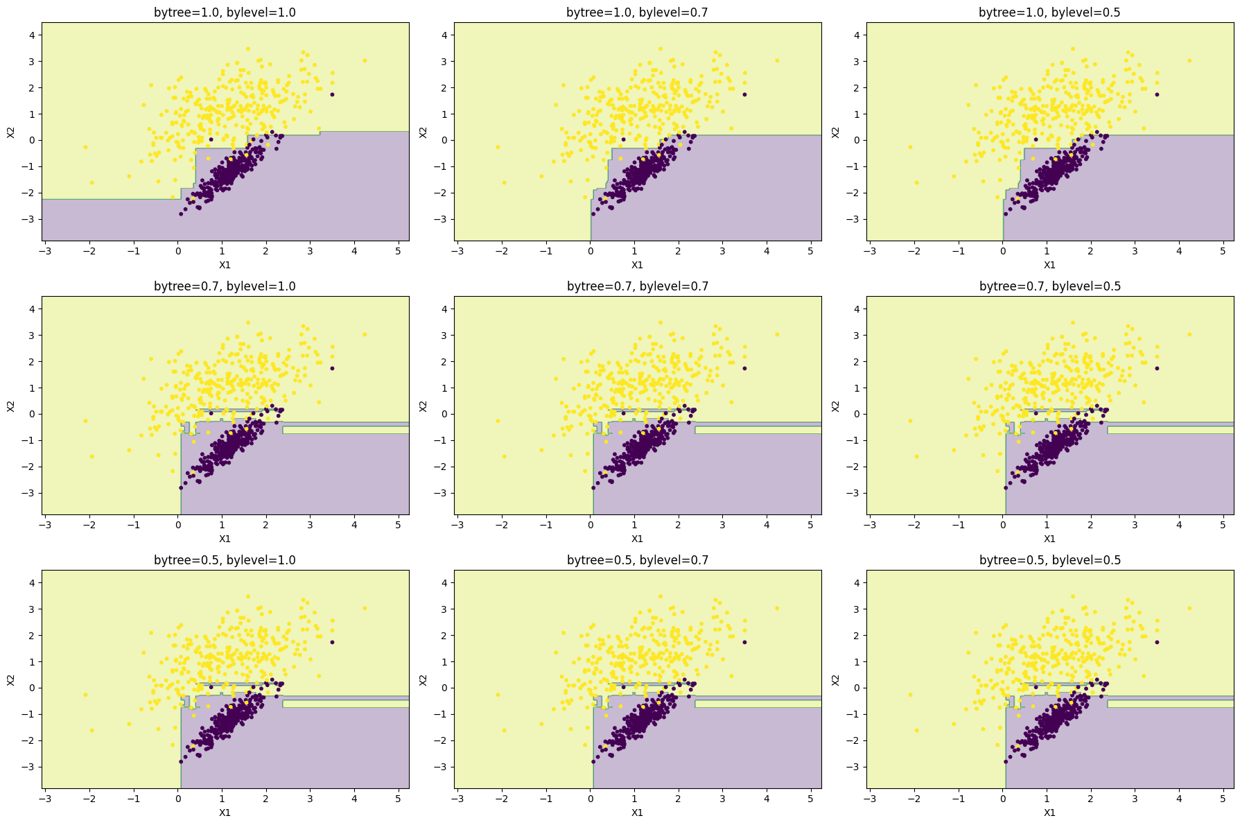
bytree
- 트리 간의 다양성 증가
- 트리 하나가 만들어지는 동안 한 번만 피처 서브셋을 랜덤하게 선택
- 하나의 트리에서는 같은 피처를 보고 분할
bylevel
- 같은 트리 안에서 다양한 구조
- 레벨마다 랜덤한 관점에서 분할 (ex. level 0에서는 f1 ~ f3만 보고 분할, level 1에서는 f3 ~ f5를 보고 분할)
reg_alpha : float
- 가중치에 대한 L1 정규화 항
- 가중치 절댓값 합을 최소화하는 규제
- 값이 커질수록 일부 트리의 잎사귀(weight)가 0이 되어 특징 선택 효과와 과적합 감소
- reg_alpha ↑ → 모델 희소(sparse)화, 일부 잎사귀 무시
reg_lambda : float
- 가중치에 대한 L2 정규화 항
- 가중치 제곱합을 최소화하는 규제
- 값이 커질수록 모든 가중치가 작아짐, 과적합 감소, 더 부드러운 모델
- reg_lambda ↑ → 모델 전체 가중치 축소, 덜 과적합
scale_pos_weight : float
- 양성 / 음성 클래스 가중치 조정
- 클래스 불균형(class imbalance)을 조정할 때 사용
- 값 > 1: positive 클래스(1)에 더 큰 가중치 → 모델이 positive를 더 잘 맞추도록 유도
- 값 < 1: positive 클래스 중요도를 낮춤 (rarely 사용)
- 불균형 비율 계산 후 적용 → scale_pos_weight = (#negative) / (#positive)
from xgboost import XGBClassifier
from sklearn.datasets import make_classification
from sklearn.model_selection import train_test_split
from sklearn.metrics import classification_report

# 극단적으로 불균형 데이터 생성 (positive 5%, negative 95%)
X, y = make_classification(
    n_samples=500,
    n_features=5,
    n_informative=3,
    n_redundant=0,
    n_clusters_per_class=1,
    weights=[0.95, 0.05],
    flip_y=0,
    random_state=42
)

X_train, X_test, y_train, y_test = train_test_split(X, y, test_size=0.2, random_state=42)

# scale_pos_weight 비교
for spw in [1, 19]:  # negative/positive = 0.95/0.05 ~ 19
    model = XGBClassifier(
        scale_pos_weight=spw,
        use_label_encoder=False,
        eval_metric='logloss',
        n_estimators=1000,
        max_depth=3,
        learning_rate=0.1,
        random_state=42
    )
    model.fit(X_train, y_train)
    y_pred = model.predict(X_test)
    print(f"=== scale_pos_weight={spw} ===")
    print(classification_report(y_test, y_pred))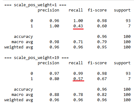
→ minority 클래스(positive)를 더 잘 맞추도록 모델이 학습
→ 모델이 minority class(positive)를 더 많이 맞추려 시도
→ Recall ↑ (positive를 놓치는 경우가 줄어듦)

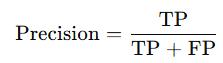
→ False Positive 증가 가능 → Precision ↓
→ 왜냐하면 모델이 positive로 더 적극적으로 예측하면서 틀린 것도 포함될 수 있음
base_score : float
- 모든 인스턴스의 초기 예측 점수, 전역 편향
- XGBoost는 잔차(residual) 학습 방식으로 트리를 쌓는데,
→ 초기 예측값 = base_score
→ 첫 번째 트리: 실제 값 - base_score 차이(잔차)를 학습
→ 두 번째 트리: 첫 번째 트리 예측값 잔차 학습
→ …
→ 즉, base_score는 첫 트리가 맞추려는 목표의 출발점 역할을 한다.
- 트리 학습 자체에는 큰 영향을 주지 않지만 학습 속도와 초기 잔차 규모에 영향
- 불균형 데이터에서 positive / negative 비율에 맞춰 주면 첫 트리가 더 안정적으로 학습
불균형 클래스에서 positive 비율이 낮은 데이터의 경우
- base_score=0.5 → 첫 트리의 잔차가 positive는 +0.5, negative는 -0.5
→ positive 영향력이 상대적으로 작음
- base_score=positive 비율 (ex. 0.1)
→ 첫 트리 잔차 positive +0.9, negative -0.1
→ 소수 클래스 영향력이 더 커짐
→ 학습 초기부터 불균형 보정
'개발 > Python' 카테고리의 다른 글
| 검정 통계량 T, 평균의 차이와 신뢰구간 (0) | 2025.09.08 |
|---|---|
| 병합적 군집분석 계산 방법 비교 (linkage) (0) | 2025.09.08 |
| 군집화 비교 (0) | 2025.09.08 |
| MAE / MAPE / MSE / RMSE / MSLE / R2 (0) | 2025.09.08 |
| Threshold 조정에 따른 Precision과 Recall 결과 (0) | 2025.09.08 |


댓글