서포트 벡터
- 데이터가 사상된 공간에서 경계선과 가장 근접한 데이터
- Support Vector가 많을수록 모델의 복잡도가 높아지고 일반화 성능이 낮아짐
- Linear SVM의 학습 결과는 선형 판별함수로 대체 가능
커널 트릭
- 원래 공간에서 선형 분류가 불가능한 경우에도, 커널을 사용하여 고차원 공간에서 선형 분류가 가능
- 고차원 속성들을 직접 생성하지 않고 비선형 패턴을 분류
- 고차원에서의 특징 추출이 어려운 경우 차원의 저주를 회피
소프트 마진(Soft Margin)
- 약간의 마진 위반을 허용하여 과적합을 방지하고, 이상치에 덜 민감하게 만든다.
- 소프트 마진 판별기는 최대 마진 분류기의 분류 마진에 대한 조건을 완화시켜 선형 분리가 불가능한 경우도 적용 가능
- 회귀에서는 마진 오류 안에서 도로 안에 가능한 많은 데이터 샘플이 들어가도록 학습

법선 벡터가 w일 때, SVM 최종 마진은
이며, SVM의 최적화 목표는 다음과 같다.

- SVM은 플러스 마진과 마이너스 마진 사이를 극대화 (+1, -1 마진 경계)
- 이상치 탐지, 패턴 인식, 자료분석 등에 사용
- 2 ~ 3개의 SVM으로 다중분류 (OvR, OvO)가 가능
- SVM의 테스트(예측) 과정은 비교적 계산량이 많다. (서포트 벡터의 개수가 많을수록 예측이 느려지는 구조적 한계)
- 중소규모의 비선형 데이터셋에 적합 (큰 데이터 셋에는 부적합)
- 스케일에 민감 / 차원의 저주에 상대적으로 덜 민감
- 신경망 기법에 비해 과적합 정도가 낮음
- 저차원, 고차원 모두 잘 작동
- C가 작으면 넓은 마진 (과대적합일 경우 C를 감소시켜 오분류를 더 허용 → 결정 경계가 부드러워짐 → 일반화 성능 ↑)
- 회귀 : C가 작으면 잘못 예측한 값에 대해 패널티 부여 → 작아질수록 회귀식이 평평
단점
- 데이터 전처리와 매개변수 설정에 따라 정확도가 달라짐
- 예측이 어떻게 이루어지는지에 대한 이해와 모델에 대한 해석이 어려움
- 대용량 데이터에 대한 모형 구축시 속도가 느리며, 메모리 할당량이 큼
sklearn.svm의 SVC / SVR 의 옵션은 다음과 같다.


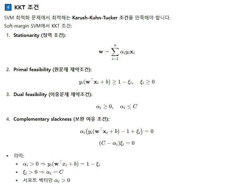
최대 마진 위의 지지벡터 조건

α가 0이면 최대 마진 바깥 쪽의 Support Vector
α가 C면 최대 마진 안 쪽의 Support Vector
하이퍼 파라미터
from sklearn.svm import SVC, SVR

SVC(
    C=1.0,
    kernel='rbf',
    degree=3,
    gamma='auto_deprecated',
    coef0=0.0,
    shrinking=True,
    probability=False,
    tol=0.001,
    cache_size=200,
    class_weight=None,
    verbose=False,
    max_iter=-1,
    decision_function_shape='ovr',
    random_state=None,
)

SVR(
    kernel='rbf',
    degree=3,
    gamma='auto_deprecated',
    coef0=0.0,
    tol=0.001,
    C=1.0,
    epsilon=0.1,
    shrinking=True,
    cache_size=200,
    verbose=False,
    max_iter=-1,
)
clf_linear = SVC(kernel='linear')

clf_poly = SVC(kernel='poly', degree=3, gamma='scale', coef0=1)

비선형 분리 문제에 효과적
고차원 공간으로 매핑해 초평면 분리
clf_rbf = SVC(kernel='rbf', gamma='scale')

clf_sigmoid = SVC(kernel='sigmoid', gamma='scale', coef0=0)

precomputed 예시
import numpy as np
from sklearn.svm import SVC
from sklearn.metrics import accuracy_score
from sklearn.model_selection import train_test_split

def rbf_kernel(X1, X2, gamma=0.1):
    # ||x - y||^2 계산 → RBF 커널
    sq_dists = np.sum(X1**2, axis=1).reshape(-1,1) \
               + np.sum(X2**2, axis=1) - 2 * X1 @ X2.T
    return np.exp(-gamma * sq_dists)

# 데이터 생성
X = np.random.randn(20, 3)
y = np.array([0]*10 + [1]*10)

# 분리
X_train, X_test, y_train, y_test = train_test_split(X, y, test_size=0.3)

# 커널 행렬 계산
K_train = rbf_kernel(X_train, X_train, gamma=0.5)
K_test = rbf_kernel(X_test, X_train, gamma=0.5)

# 학습
clf = SVC(kernel='precomputed')
clf.fit(K_train, y_train)

# 예측
pred = clf.predict(K_test)
print("Accuracy:", accuracy_score(y_test, pred))
C vs gamma
C (Regularization Parameter)
- 오류 항에 대한 페널티 매개변수
- 오분류를 얼마나 허용할지를 결정하는 규제(regularization) 파라미터
- 즉, 결정 경계를 단단하게 할지(C 큼) vs 느슨하게 할지(C 작음)를 조절
C가 크면 (C ↑)
- 오분류 허용 X → 각 데이터 포인트를 최대한 정확히 분류하려 함
- 결정 경계가 복잡해지고 과적합(overfitting) 가능성 ↑
C가 작으면 (C ↓)
- 일부 오분류 허용 → 더 단순한 경계 형성
- 결정 경계가 부드럽고 일반화 능력 ↑
gamma (Kernel Coefficient, for RBF/poly/sigmoid kernel)
- 'rbf', 'poly', 'sigmoid' 커널의 계수
- 현재 기본값 'auto'는 1 / n_features를 사용
- gamma='scale'를 지정하면 1 / (n_features * X.var())가 사용
- 하나의 학습 데이터가 미치는 영향 범위를 조절
- 즉, 결정 경계의 곡률(curvature)을 제어
gamma가 크면 (γ ↑)
- 각 샘플의 영향 범위가 작음
- 국소적으로만 작용 → 결정 경계가 매우 복잡
- 과적합 위험 ↑
gamma가 작으면 (γ ↓)
- 각 샘플의 영향 범위가 넓음
- 전체적으로 부드러운 경계 → 단순한 모델
- 과소적합 위험 ↑
SVC
import numpy as np
import matplotlib.pyplot as plt
from sklearn.svm import SVC
from sklearn.datasets import make_moons

# 2차원 분류 데이터 생성
X, y = make_moons(n_samples=200, noise=0.2, random_state=42)

# C와 gamma 후보
C_values = [0.1, 1, 10]
gamma_values = [0.1, 1, 10]

plt.figure(figsize=(12, 12))

# 3x3 그리드로 그리기
for i, C in enumerate(C_values):
    for j, gamma in enumerate(gamma_values):
        svc = SVC(C=C, gamma=gamma)
        svc.fit(X, y)

        # 결정 경계 그리기
        x_min, x_max = X[:, 0].min() - 0.5, X[:, 0].max() + 0.5
        y_min, y_max = X[:, 1].min() - 0.5, X[:, 1].max() + 0.5
        xx, yy = np.meshgrid(np.linspace(x_min, x_max, 200),
                             np.linspace(y_min, y_max, 200))
        Z = svc.predict(np.c_[xx.ravel(), yy.ravel()]).reshape(xx.shape)

        plt.subplot(3, 3, i*3 + j + 1)
        plt.contourf(xx, yy, Z, alpha=0.3, cmap=plt.cm.coolwarm)
        plt.scatter(X[:, 0], X[:, 1], c=y, s=30, cmap=plt.cm.coolwarm, edgecolors='k')
        plt.title(f"C={C}, gamma={gamma}")
        plt.xlim(xx.min(), xx.max())
        plt.ylim(yy.min(), yy.max())

plt.tight_layout()
plt.show()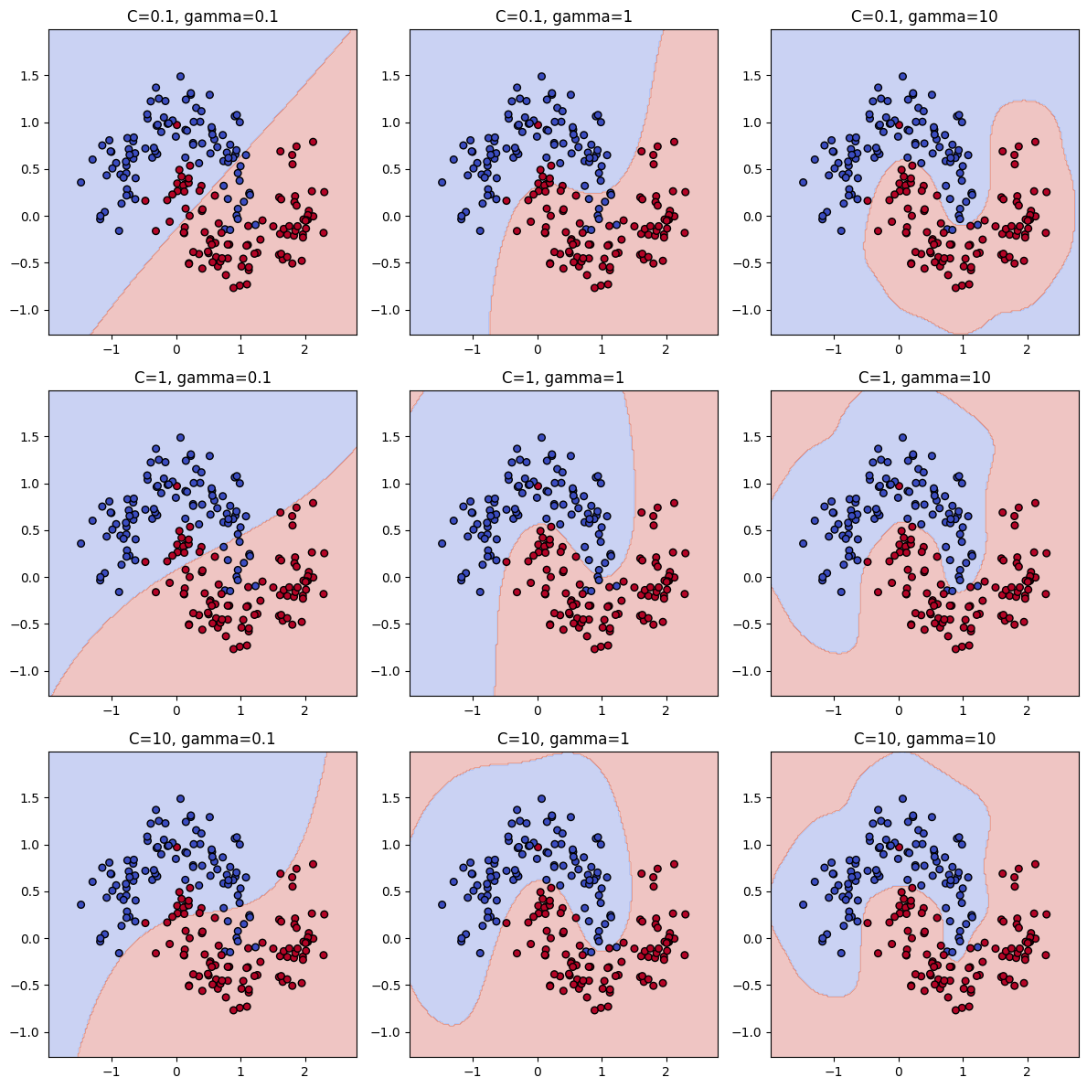
SVR
import numpy as np
import matplotlib.pyplot as plt
from sklearn.svm import SVR

# 샘플 데이터 생성
X = np.sort(5 * np.random.rand(100, 1), axis=0)
y = np.sin(X).ravel() + 0.2 * np.random.randn(100)

# C와 gamma 후보
C_values = [0.1, 1, 10]
gamma_values = [0.1, 1, 10]

plt.figure(figsize=(12, 12))
X_plot = np.linspace(0, 5, 100).reshape(-1, 1)

# 3x3 그리드로 그리기
for i, C in enumerate(C_values):
    for j, gamma in enumerate(gamma_values):
        svr = SVR(C=C, gamma=gamma)
        svr.fit(X, y)
        y_pred = svr.predict(X_plot)

        plt.subplot(3, 3, i*3 + j + 1)
        plt.scatter(X, y, color='darkorange', label='data')
        plt.plot(X_plot, y_pred, color='navy', lw=2, label='SVR fit')
        plt.title(f"C={C}, gamma={gamma}")
        plt.ylim(-2, 2)
        if i == 2 and j == 0:
            plt.legend()

plt.tight_layout()
plt.show()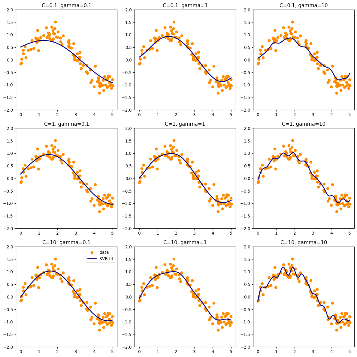
tol : float
- 학습 종료 기준에 대한 허용 오차
- 손실 감소량이 tol보다 작아지면 더 학습해도 변화가 거의 없다라고 판단하고 종료
epsilon
- ε = "이 정도 차이는 오차로 취급하지 않겠다는 허용 범위"
- ε-SVR은 epsilon-tube라는 오차 허용 범위를 가짐.
- 예측값과 실제값의 차이가 ε 이하 → 오차를 완전히 무시 (=패널티 없음)
- 이 영역 안에 있는 점은 서포트 벡터가 되지 않고 모델 파라미터 최적화에 영향을 거의 주지 않는다.
epsilon이 작을수록
- 허용 오차가 거의 없다 → 아주 예민해짐
→ 작은 차이도 오차로 인식
→ 더 많은 점이 서포트 벡터가 됨
→ 모델이 데이터를 더 정확하게 따라감
→ 과적합(overfitting) 가능성 ↑
epsilon이 클수록
- 오차 허용 범위가 넓어짐
→ 작은 차이는 무시됨
→ 서포트 벡터 수가 줄어듦
→ 모델이 더 부드러워짐
→ 과적합 방지 및 일반화 성능 ↑
import numpy as np
import matplotlib.pyplot as plt
from sklearn.svm import SVR

# 데이터 생성
np.random.seed(0)
X = np.sort(5 * np.random.rand(100, 1), axis=0)
y = np.sin(X).ravel() + 0.2 * np.random.randn(100)

epsilons = [0.01, 0.5, 1]

fig, axes = plt.subplots(1, 3, figsize=(15, 4))

for ax, eps in zip(axes, epsilons):
    svr = SVR(kernel='rbf', epsilon=eps, C=10, gamma=0.5)
    y_pred = svr.fit(X, y).predict(X)

    ax.scatter(X, y)
    ax.plot(X, y_pred)
    ax.set_title(f"epsilon = {eps}")
    ax.set_xlabel("X")
    ax.set_ylabel("y")

plt.tight_layout()
plt.show()
→ ε가 작을수록 과대적합이 되는 것을 알 수 있다.
shrinking : bool
- 수축(shrinking) 휴리스틱을 사용할지 여부
- SMO에서 계산 속도를 높이기 위해 활성화되는 근사 기법
* SMO : Support Vector Machine의 Quadratic Programming 문제를 푸는 Sequential Minimal Optimization 알고리즘
shrinking=True (기본값)
- 학습 도중 일부 라그랑주 승수(dual coefficients)를 임시로 제외시켜 계산량을 줄임
- 나중에 필요하면 다시 포함시켜 최종 최적화를 진행
- 큰 데이터셋에서 학습 속도가 빨라짐
- 데이터가 작거나 정확도가 최우선
shrinking=False
- 모든 데이터를 항상 포함
- 더 정확할 수 있지만 큰 데이터에서는 느림
- 데이터가 크고 학습 속도가 중요
Attributes
SVC
    support_ : array-like, shape = [n_SV]
        Indices of support vectors.

    support_vectors_ : array-like, shape = [n_SV, n_features]
        Support vectors.

    n_support_ : array-like, dtype=int32, shape = [n_class]
        Number of support vectors for each class.

    dual_coef_ : array, shape = [n_class-1, n_SV]
        Coefficients of the support vector in the decision function.
        For multiclass, coefficient for all 1-vs-1 classifiers.
        The layout of the coefficients in the multiclass case is somewhat
        non-trivial. See the section about multi-class classification in the
        SVM section of the User Guide for details.

    coef_ : array, shape = [n_class * (n_class-1) / 2, n_features]
        Weights assigned to the features (coefficients in the primal
        problem). This is only available in the case of a linear kernel.

        `coef_` is a readonly property derived from `dual_coef_` and
        `support_vectors_`.

    intercept_ : array, shape = [n_class * (n_class-1) / 2]
        Constants in decision function.

    fit_status_ : int
        0 if correctly fitted, 1 otherwise (will raise warning)

    probA_ : array, shape = [n_class * (n_class-1) / 2]
    probB_ : array, shape = [n_class * (n_class-1) / 2]
        If probability=True, the parameters learned in Platt scaling to
        produce probability estimates from decision values. If
        probability=False, an empty array. Platt scaling uses the logistic
        function
        ``1 / (1 + exp(decision_value * probA_ + probB_))``
        where ``probA_`` and ``probB_`` are learned from the dataset [2]_. For
        more information on the multiclass case and training procedure see
        section 8 of [1]_.
SVR
    support_ : array-like, shape = [n_SV]
        Indices of support vectors.

    support_vectors_ : array-like, shape = [nSV, n_features]
        Support vectors.

    dual_coef_ : array, shape = [1, n_SV]
        Coefficients of the support vector in the decision function.

    coef_ : array, shape = [1, n_features]
        Weights assigned to the features (coefficients in the primal
        problem). This is only available in the case of a linear kernel.

        `coef_` is readonly property derived from `dual_coef_` and
        `support_vectors_`.

    intercept_ : array, shape = [1]
        Constants in decision function.
support_
- 서포트 벡터가 된 샘플의 인덱스(index) 리스트
- 원본 데이터에서 어떤 샘플들이 결정 경계를 형성하는 데 중요한 역할을 했는지 알려준다.
support_vectors_
- 서포트 벡터의 실제 데이터 값
- X[support_] == support_vectors_
dual_coef_
- 결정 함수에서 서포트 벡터의 계수
coef_
- 특성에 할당된 가중치 (원 문제에서의 계수)
- 선형 커널인 경우에만 사용 가능
'개발 > Python' 카테고리의 다른 글
| 데이터 범주화, 구간화 (1) | 2025.08.15 |
|---|---|
| 정규성 검정 (2) | 2025.08.15 |
| 선형회귀모형의 변수 선택 (후진제거법, 전진선택법) (1) | 2025.08.14 |
| 병합적 군집분석 결과를 다른 데이터 샘플에 적용하기 (3) | 2025.08.13 |
| Pandas 전처리 - 이상치 탐지 (4) | 2025.08.12 |


댓글