마할라노비스 거리
- 공분산으로 표준화된 거리
- 각 변수의 단위 차이나 서로 간 상관관계를 고려해서 거리를 계산
- 다변량 정규성 검정
- 군집 분석에서 데이터 중심과 거리 측정
- 이상치 탐지 (LOF, Mahalanobis outlier) :
마할라노비스 거리가 크면 평균에서 멀리 떨어짐 → 일반적인 분포에서 벗어남
- 데이터가 서로 상관관계가 있거나 각 변수의 분산이 다를 때는 유클리드 거리로만 비교하면 왜곡이 생길 수 있다.
ex. 몸무게가 변동이 큰데 유클리드 거리만 쓰면 키보다 몸무게 차이가 지나치게 크게 반영
→ 마할라노비스 거리를 사용
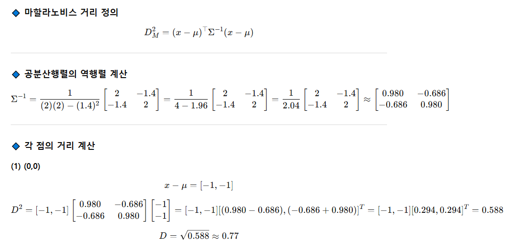
수식

특징
- 단위 무관(Unitless) : 변수 단위가 달라도 영향을 최소화
- 상관관계 반영 : 변수 간 상관이 높으면, 그 방향의 거리는 상대적으로 작게 계산
- 이상치 탐지(Outlier Detection)에 유용 : 평균에서 멀리 떨어진 점이 얼마나 "분포를 벗어났는지" 판단 가능
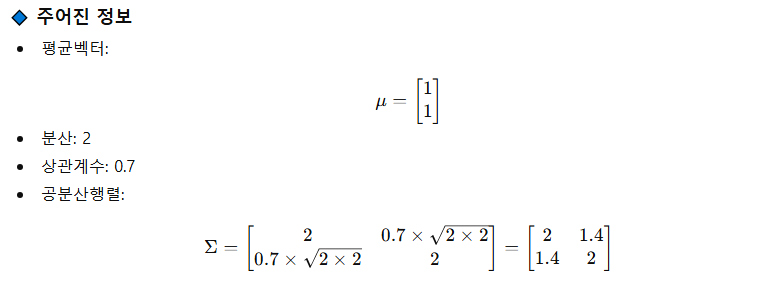
X, Y 평균이 1, 분산이 2이고 서로의 상관계수는 0.7일 때, 각 좌표와의 거리를 계산하시오.
→ (0, 0) / (2, 0) / (2, 1) / (2, 2)
...
import numpy as np
import matplotlib.pyplot as plt
from scipy.spatial import distance
from matplotlib.patches import Ellipse

# 평균과 공분산 설정
mean = np.array([1, 1])
cov = np.array([[2, 1.4],
                [1.4, 2]])

# 후보 점들
points = np.array([
    [0, 0],
    [2, 0],
    [2, 1],
    [2, 2]
])
labels = ['(0,0)', '(2,0)', '(2,1)', '(2,2)']

# 역공분산행렬
inv_cov = np.linalg.inv(cov)

# 마할라노비스 거리 계산
distances = []
for p in points:
    d = distance.mahalanobis(p, mean, inv_cov)
    distances.append(d)
    print(f"{p}: Mahalanobis distance = {d:.3f}")

# 가장 먼 점
max_idx = np.argmax(distances)
print(f"\n가장 먼 점: {labels[max_idx]} (거리={distances[max_idx]:.3f})")

# --- 시각화 ---
fig, ax = plt.subplots(figsize=(6, 6))

# 점 표시
for i, p in enumerate(points):
    ax.scatter(*p, label=f"{labels[i]} (D={distances[i]:.2f})", s=100)
ax.scatter(*mean, color='red', marker='x', s=100, label='Mean (1,1)')

# 등거리 타원 (공분산 기반)
eigvals, eigvecs = np.linalg.eigh(cov)
for n_std in [1, 2]:
    width, height = 2 * n_std * np.sqrt(eigvals)
    angle = np.degrees(np.arctan2(*eigvecs[:, 0][::-1]))
    ellipse = Ellipse(mean, width, height, angle, edgecolor='gray', facecolor='none', linestyle='--', alpha=0.7)
    ax.add_patch(ellipse)

# 꾸미기
ax.legend()
ax.set_xlim(-1, 4)
ax.set_ylim(-1, 4)
ax.set_xlabel('X')
ax.set_ylabel('Y')
ax.set_title('Mahalanobis Distance from Mean (1,1)')
ax.grid(True)
plt.show()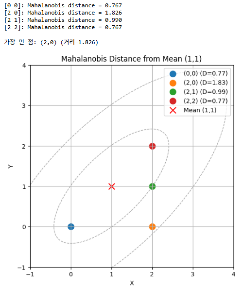
X, Y 평균이 0, 분산이 1이고 서로의 상관계수는 0.7일 때, 각 좌표와의 거리를 계산하시오.
→ (0, 0) / (2, 0) / (2, 1) / (2, 2)
import numpy as np
import matplotlib.pyplot as plt
from scipy.spatial import distance
from matplotlib.patches import Ellipse

# 평균과 공분산 설정
mean = np.array([0, 0])
cov = np.array([[1, 0.7],
                [0.7, 1]])

# 후보 점들
points = np.array([
    [0, 0],
    [2, 0],
    [2, 1],
    [2, 2]
])
labels = ['(0,0)', '(2,0)', '(2,1)', '(2,2)']

# 역공분산행렬
inv_cov = np.linalg.inv(cov)

# 마할라노비스 거리 계산
distances = []
for p in points:
    d = distance.mahalanobis(p, mean, inv_cov)
    distances.append(d)
    print(f"{p}: Mahalanobis distance = {d:.3f}")

# 가장 먼 점
max_idx = np.argmax(distances)
print(f"\n가장 먼 점: {labels[max_idx]} (거리={distances[max_idx]:.3f})")

# --- 시각화 ---
fig, ax = plt.subplots(figsize=(6, 6))

# 점 표시
for i, p in enumerate(points):
    ax.scatter(*p, label=f"{labels[i]} (D={distances[i]:.2f})", s=100)
ax.scatter(*mean, color='red', marker='x', s=100, label='Mean (0,0)')

# 등거리 타원 (공분산 기반)
eigvals, eigvecs = np.linalg.eigh(cov)
for n_std in [1, 2]:
    width, height = 2 * n_std * np.sqrt(eigvals)
    angle = np.degrees(np.arctan2(*eigvecs[:, 0][::-1]))
    ellipse = Ellipse(mean, width, height, angle, edgecolor='gray', facecolor='none', linestyle='--', alpha=0.7)
    ax.add_patch(ellipse)

# 꾸미기
ax.legend()
ax.set_xlim(-1, 3)
ax.set_ylim(-1, 3)
ax.set_xlabel('X')
ax.set_ylabel('Y')
ax.set_title('Mahalanobis Distance from Mean (0,0)')
ax.grid(True)
plt.show()
X, Y 평균이 3, 분산이 5이고 서로의 상관계수는 0.5일 때, 각 좌표와의 거리를 계산하시오.
→ (0, 0) / (2, 0) / (2, 1) / (2, 2)
import numpy as np
import matplotlib.pyplot as plt
from scipy.spatial import distance
from matplotlib.patches import Ellipse

# 평균과 공분산 설정
mean = np.array([3, 3])
var = 5
rho = 0.5
cov = np.array([[var, rho * var],
                [rho * var, var]])

# 후보 점들
points = np.array([
    [0, 0],
    [2, 0],
    [2, 1],
    [2, 2]
])
labels = ['(0,0)', '(2,0)', '(2,1)', '(2,2)']

# 역공분산행렬
inv_cov = np.linalg.inv(cov)

# 마할라노비스 거리 계산
distances = []
for p in points:
    d = distance.mahalanobis(p, mean, inv_cov)
    distances.append(d)
    print(f"{p}: Mahalanobis distance = {d:.3f}")

# 가장 먼 점
max_idx = np.argmax(distances)
print(f"\n가장 먼 점: {labels[max_idx]} (거리={distances[max_idx]:.3f})")

# --- 시각화 ---
fig, ax = plt.subplots(figsize=(6, 6))

# 점 표시
for i, p in enumerate(points):
    ax.scatter(*p, label=f"{labels[i]} (D={distances[i]:.2f})", s=100)
ax.scatter(*mean, color='red', marker='x', s=100, label='Mean (3,3)')

# 등거리 타원 (공분산 기반)
eigvals, eigvecs = np.linalg.eigh(cov)
for n_std in [1, 2]:
    width, height = 2 * n_std * np.sqrt(eigvals)
    angle = np.degrees(np.arctan2(*eigvecs[:, 0][::-1]))
    ellipse = Ellipse(mean, width, height, angle, edgecolor='gray', facecolor='none', linestyle='--', alpha=0.7)
    ax.add_patch(ellipse)

# 꾸미기
ax.legend()
ax.set_xlim(-1, 6)
ax.set_ylim(-1, 6)
ax.set_xlabel('X')
ax.set_ylabel('Y')
ax.set_title('Mahalanobis Distance from Mean (3,3)')
ax.grid(True)
plt.show()
scipy.spatial.distance의 mahalanobis로도 계산할 수 있다.
import numpy as np
from scipy.spatial.distance import mahalanobis

# 평균과 공분산 행렬, 상관계수
mean = np.array([3, 3])
var = 5
rho = 0.5
cov = np.array([[var, rho * var],
                [rho * var, var]])

# 공분산 행렬의 역행렬
inv_cov = np.linalg.inv(cov)

# 후보 좌표들
points = {
    "1) (0, 0)": np.array([0, 0]),
    "2) (2, 0)": np.array([2, 0]),
    "3) (2, 1)": np.array([2, 1]),
    "4) (2, 2)": np.array([2, 2]),
}

# 거리 계산
distances = {}
for label, point in points.items():
    dist = mahalanobis(point, mean, inv_cov)
    distances[label] = dist

# 출력
for label, dist in sorted(distances.items(), key=lambda x: -x[1]):
    print(f"{label}: Mahalanobis 거리 = {dist:.4f}")

# 1) (0, 0): Mahalanobis 거리 = 1.5492
# 2) (2, 0): Mahalanobis 거리 = 1.3663
# 3) (2, 1): Mahalanobis 거리 = 0.8944
# 4) (2, 2): Mahalanobis 거리 = 0.516'개발 > Python' 카테고리의 다른 글
| 라벨 스무딩 (Label Smoothing) (0) | 2025.10.25 |
|---|---|
| 가설검정 (0) | 2025.10.25 |
| 로버스트 피팅 (0) | 2025.10.25 |
| 하이퍼 파라미터 튜닝 (0) | 2025.10.25 |
| 기본 문법 (0) | 2025.10.25 |
댓글